Introducing fasttransform, a Python library that makes data transformations reversible and extensible through the power of multiple dispatch.
technical
Author
Rens Dimmendaal, Hamel Husain, & Jeremy Howard
Published
February 20, 2025
fasttransform: Reversible Pipelines Made Simple
Introducing fasttransform, a Python library that makes data transformations reversible and extensible through the power of multiple dispatch.
“How did this image get misclassified?”
If you’ve ever trained a machine learning model, you know what comes next: the frustrating journey of trying to understand what your model actually saw. You dig through layers of transformations - normalizations, resizes, augmentations - only to realize you’ll need to write inverse functions just to see your data again. It’s so painful that many of us skip it altogether, debugging our models based on abstract numbers rather than actual data.
Or as OpenAI’s Greg Brockman puts it:
Greg Brockman tweet: “Manual inspection of data has probably the highest value-to-prestige ratio of any activity in machine learning.”
Let’s look at what you might be missing. Here’s a simple example using fastai:
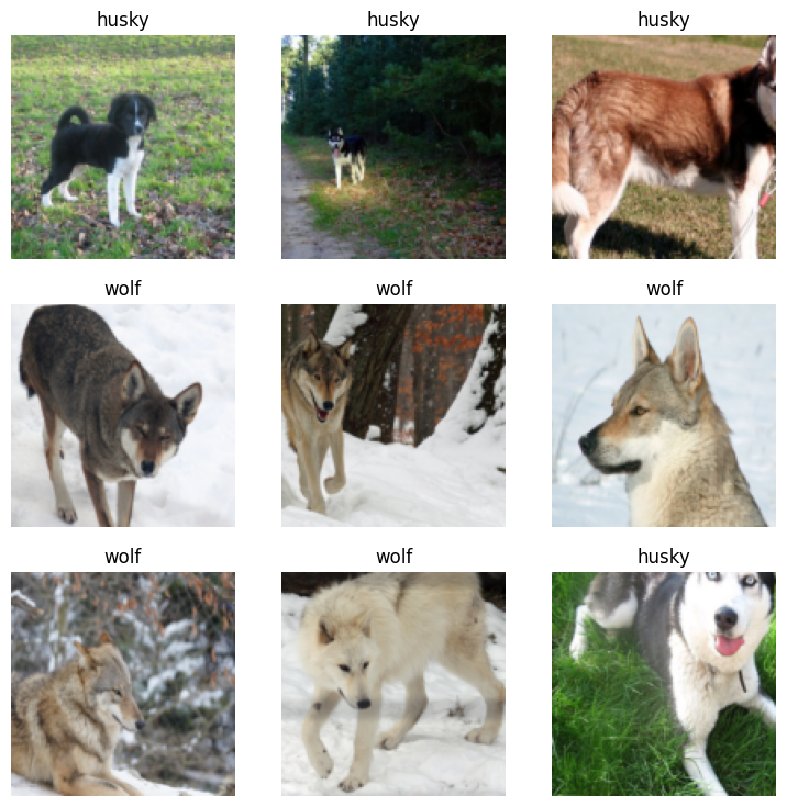
from fastai.vision.allimport*dls = ImageDataLoaders.from_folder( Path("./huskies_vs_wolves/"), item_tfms=RandomResizedCrop(128, min_scale=0.35), batch_tfms=Normalize.from_stats(*imagenet_stats))dls.show_batch() # One line to see our data
show_batch makes it easy to take a look at your data after has been transformed
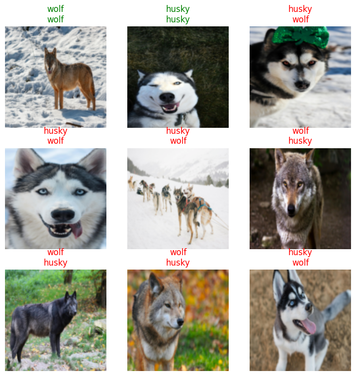
learn = Learner(dls, xresnet34(n_out=2), metrics=accuracy)learn.fit_one_cycle(5, 0.0015)learn.show_results() # One line to see predictions
show_results lets you inspect your predictions immediately after training your model. The prediction labels (0/1) are also automatically transformed back to their string representation.
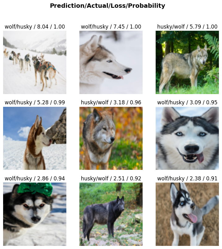
# Two lines to see the model's biggest mistakesinterp = Interpretation.from_learner(learn)interp.plot_top_losses(9)
plot_top_losses visualizes where the model is “most confidently wrong” which teaches us about the most glaring issues.
With just these four lines, we discover something fascinating: our “wolf detector” isn’t detecting wolves at all - it’s detecting snow! Look at the training data: wolves in snow, huskies in forests. Then look at the predictions: the model fails whenever we flip the backgrounds. Without being able to easily visualize our data, we might never have caught this obvious flaw.
The LIME technique visualizes how the model focuses on snowy backgrounds to make its predictions
While sophisticated interpretability techniques like LIME1 can beautifully visualize what parts of the image your model is focusing on (as shown above), often the most valuable insights come from simply being able to look at your data with your own eyes. In this case, a quick visual inspection revealed an obvious dataset bias just as well.
How does fastai do this? Well, it uses Transform – a deceptively simple yet powerful idea that’s been hiding inside fastcore’s codebase. Today, we’re excited to announce that we’ve moved it to its own library: fasttransform, because we believe its applications may go beyond machine learning.
Whether you’re working with images, text, time series, or any other data that needs processing, fasttransform offers a simple promise: if you can transform your data one way, you should be able to transform it back just as easily. No more writing inverse functions, no more losing sight of your data.
Let’s see how it works.
Problem #1: One-Way Transforms
Ever tried to debug a machine learning pipeline by looking at your data? It usually goes something like this:
Load your data
Apply some transformations
Try to figure out what went wrong
Realize you can’t actually see what your model is seeing
Spend the next hour writing inverse functions
Give up and debug with print statements instead
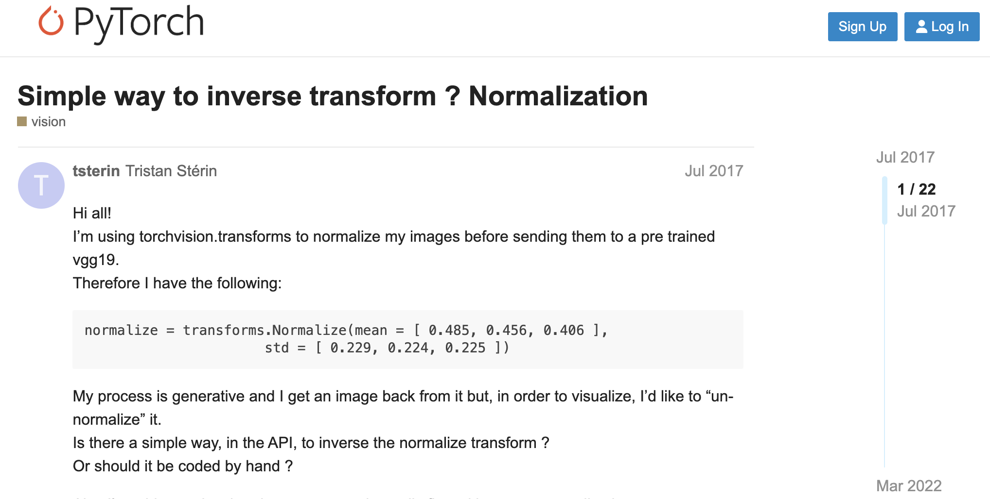
Let’s make this concrete with a simple example: normalizing an image with PyTorch:
from torchvision import transforms as Ttransforms_pt = T.Compose([ T.Resize(256), T.CenterCrop(224), T.ToTensor(), T.Normalize(*imagenet_stats)])# Load and transform an imageimg = Image.open("./huskies_vs_wolves/train/husky/husky_0.jpeg")img_transformed = transforms_pt(img)# Try to look at what we did...show_image(img_transformed);
Clipping input data to the valid range for imshow with RGB data ([0..1] for floats or [0..255] for integers). Got range [-2.1007793..2.2489083].
Normalization is a crucial preprocessing step that scales pixel values to have similar ranges (typically mean=0 and standard deviation=1), which helps neural networks train more effectively.
However, the normalization doesn’t really make this picture suitable for inspection with human eyes. To fix this, we need to manually write an inverse transform:
def decode_pt(tensor, mean, std):"""Decode a normalized PyTorch tensor back to RGB range""" out = tensor.clone() # Clone to avoid modifying originalfor t, m, s inzip(out, mean, std): t.mul_(s).add_(m) # Denormalize out = out.mul(255).clamp(0, 255).byte() # Scale back to RGBreturn outimg_decoded = decode_pt(img_transformed, *imagenet_stats)show_image(img_decoded);
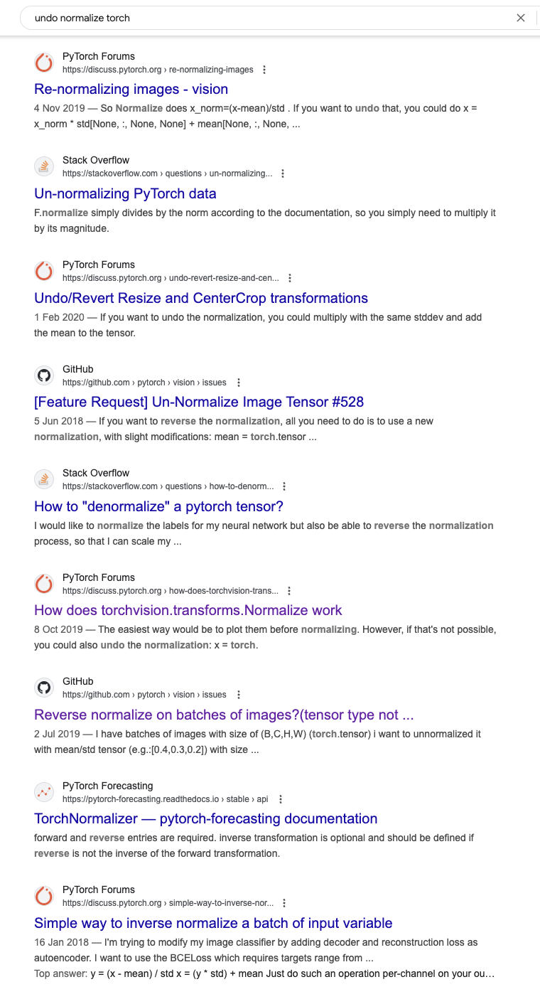
And this is not some obscure problem. This has been a pain point of many ML practicioners for years:
And this was just for a simple normalization. In real projects, you’re probably dealing with: - Segmentation masks that need to be transformed in sync with images - Text data with tokenization, padding, and special tokens - Time series with sliding windows, normalization, and encoding
Each transformation adds another layer of complexity to unwind. And here’s the worst part: because it’s so painful to look at your transformed data, many of us just… don’t. We end up debugging our models based on abstract numbers rather than actual data, hoping our transformations are doing what we think they’re doing.
Remember how easy it was in our fastai example to see exactly what the model was seeing? That’s not magic - it’s the power of reversible transforms. Let’s see how fasttransform makes this possible.
A Better Way: reversible pipelines
Here’s how fastai handles the same pipeline as the pytorch example of the previous section:
Clipping input data to the valid range for imshow with RGB data ([0..1] for floats or [0..255] for integers). Got range [-2.0836544..2.2317834].
# But now the magic:img_decoded = transforms_ft.decode(img_transformed)show_image(img_decoded[0]);# That's better!
That’s it. No manual inverse functions. No remembering means and standard deviations. Just .decode() and we’re back to something we can actually look at.
fasttransform brings this same capability to your own code. The key insight is that for any transformation you want to apply, you probably already know how to undo it. Let’s look at how this works internally.
How it works: .decode()
The core idea behind fasttransform is simple: pair a transformation with its inverse.
Here’s how you write a reversible normalization transform:
By defining both encodes and decodes, fasttransform automatically knows how to reverse your transformations. Compare this to our earlier PyTorch example - instead of writing separate forward and inverse functions, we keep them together where they belong.
You might notice the peculiar naming - encodes and decodes with an ‘s’. We’ll explain why later, but it has everything to do with how fasttransform handles different types of data automatically.
When you call decode(), fasttransform is smart about which transforms to reverse. Some transforms, like loading an image or resizing it, don’t need to be undone, you actually want to see what the model sees! Others, like normalization, need to be reversed to be human-readable.
How do you do this? Well, only define a .decodes method if the transform needs to be inverted!
The introduction’s plotting functions used exactly this functionality to turn the transformed inputs back into a human interpretable state.
Problem #2: Dealing with multiple types
We’ve seen how making transforms reversible makes it easier to look at your data. But there’s another challenge when working with transforms: different types of data need different transformations.
You see this most often where your inputs and your labels need different transforms. Here the same principle applies. We’d like to keep all those transforms in one place together because we want to be able to undo both of them. For example, we want to transform our categorical labels from strings to integers and back to strings again for human readability. But we don’t want to maintain separate transform pipelines for the inputs and the outputs.
To understand why this is a problem, let’s look at how PyTorch - one of the most popular deep learning frameworks - handles this situation. Here’s an example from the tutorial showing a typical custom dataset:
The transforms for images and labels are separately defined and provided to the dataset class. This separation might seem reasonable at first, but it creates two problems:
When we want to reverse the transforms, we have to remember to reverse both pipelines
When we have transforms that need to apply to both input and target we have to maintain them in two places (e.g. image and mask resizing for image segmentation)
Let’s see how fasttransform makes this easier.
A better way: one pipeline for both input and outputs
Here’s where fasttransform’s approach shines: instead of juggling separate pipelines, it handles both your image and its label in a single transform. When you pass a tuple to a transform, it only applies the relevant transforms. This might sound like a small thing, but it’s a game-changer for real-world machine learning work.
Let’s see this in action.
First, we’ll create a function that loads both an image and its label:
But we’re not done yet! Those string labels (“husky”, “wolf”) need to be converted to numbers for our model. In PyTorch, we’d need a separate transform pipeline for this. With fasttransform, we just add another transform that only applies to strings:
class StrCategorize(Transform):def__init__(self, vocab):self.vocab = vocabself.s2i = {s:i for i,s inenumerate(vocab)}self.i2s = {i:s for i,s inenumerate(vocab)}def encodes(self, s:str): returnself.s2i[s]def decodes(self, i:int): returnself.i2s[i]transforms_ft = Pipeline([ load_img_and_label, Resize(256,method="squish"), Resize(224,method="crop"), ToTensor(), IntToFloatTensor(), Normalize.from_stats(*imagenet_stats, cuda=False), StrCategorize(vocab=['husky','wolf']), # <-- Transform is just for the target label])out = transforms_ft(fpath)print((out[0][0,:2,:2,:2], out[1]))
Next we’ll show another example that shows why it’s crucial to keep those transforms in one place: image segmentation.
In segmentation, you’re trying to identify specific regions in an image - like finding a husky in a photo. But here’s the tricky part: both your input image AND your target mask need to be transformed in exactly the same way. And that gets tricky when you use random transforms as a form of data augmentation. To illustrate, if you apply a randomized crop to your image, then you better crop that mask in the exact same way!
Let’s see what this looks like in practice. First, we define a new function which loads both images and their corresponding mask:
Now, if we want to randomly crop both the image and the mask (a common augmentation technique), they need to be cropped in exactly the same way. If they’re not aligned then your whole training data becomes nonsense.
Here’s how fasttransform handles this:
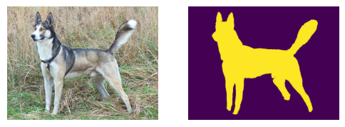
transforms_ft = Pipeline([ load_img_msk, # <-- New load func for img and mask RandomResizedCrop(200), # Applied to both img and mask ToTensor(), # Applied to both img and mask IntToFloatTensor(), # Only applied to img Normalize.from_stats(*imagenet_stats,cuda=False) # Only applied to img])out = transforms_ft(fn)outshow_images((out[0][0], out[1]))
Clipping input data to the valid range for imshow with RGB data ([0..1] for floats or [0..255] for integers). Got range [-1.8096584..2.64].
And voila, both the source image and the target mask have been transformed in identical ways.
If these transforms were stored in different pipelines then it would have been a lot harder to keep these transforms in sync. Especially because there was a randomized element in the transform.
At this point you might be thinking: “This is pretty great - one pipeline handling different types of data, applying on the the relevant transforms where needed. But how does it actually work?”
Well, let’s dive into that next!
How it works: multiple dispatch
The secret sauce that makes Transforms only apply to relevant data types is something called multiple dispatch. Don’t worry if you haven’t heard of it before - it’s a powerful programming concept that’s popular in languages like Julia2, but relatively unknown in Python.
Think of multiple dispatch like having different versions of the same function, each designed to handle specific types of data. When you call the function, Python automatically picks the right version based on what you give it.
Python provides an implementation limited to single argument functions out of the box:
from functools import singledispatch@singledispatchdef greet(x): return"Hello stranger!"@greet.registerdef _(x:str): returnf"Hello {x}!"@greet.registerdef _(x:int): returnf"Hello number {x}!"greet(None), greet("Alice"), greet(42)
('Hello stranger!', 'Hello Alice!', 'Hello number 42!')
Multiple dispatch extends this idea to functions with multiple arguments. While Python’s built-in tools only handle single argument dispatch, the plum library provides true multiple dispatch for any number of arguments. Here’s a simple example to illustrate the concept:
from plum import dispatchclass Dog: passclass Cat: pass@dispatchdef greet(a: Cat, b: Dog):return"Hiss!"@dispatchdef greet(a: Dog, b: Cat):return"Grrrr..."# Let's try it outcat, dog = Cat(), Dog()print(greet(cat, dog)) # "Hiss!"print(greet(dog, cat)) # Grrrr...
Hiss!
Grrrr...
Transform uses plum’s multiple dispatch capabilities internally, but the core idea is the same: the right function is called based on the runtime data types it receives. This is what allows a single pipeline to handle images, labels, masks, and other types of data.
There are three different ways you can define type-specific behavior in your transforms, each suited to different situations. Let’s look at each one in turn.
The simplest way to create a transform is to pass it functions directly. This is great for quick experiments or one-off transforms:
You might use this approach when you’re prototyping or when you don’t need to reuse the transform elsewhere in your code. But for more structured code, you’ll probably want to create a proper class…
Subclassing Transform gives you a more organized way to handle different types:
Notice something interesting here: in a regular Python class, you can’t define the same method multiple times. But when subclassing from Transform, you can!
The encodes method is automatically set up for multiple dispatch, so Python knows which version to call based on the input type.
But there’s one more way to define transforms, which is particularly useful when you want to extend an existing transform…
# Method 3: Extend with decorators@MyTransformdef encodes(self, x: float): returnf"encoded float: {x=}"# Now our transform handles three types!my_transform(("hello", 42, 6.28))
This decorator syntax is incredibly useful in real-world applications.
For instance, in fastai, the Normalize transform is defined in the core library to handle images, but other modules can extend it to work with new types:
# In fastai.data.transforms:class Normalize(Transform): ... # handles image normalization# In fastai.tabular.core:@Normalizedef encodes(self, x: pd.DataFrame): ... # adds DataFrame support
This plugin-like architecture means anyone can extend existing transforms to work with new types of data, without modifying the original code. That’s the power of multiple dispatch in action!
The real power shows up when code is reused and extended in the ecosystem around fastai. Libraries like fastxtend add support for new data types without modifying the original code. Without multiple dispatch, they’d face a classic inheritance problem. Instead, with fasttransform, they can simply register new behaviors for existing transforms.
Conclusion
We’ve seen how fasttransform solves two fundamental problems in data processing:
Making transforms reversible through paired encode/decode methods
Handling different data types through multiple dispatch
While these ideas grew out of fastai’s deep learning needs, their applications extend far beyond. Whether you’re processing images, text, time series, or quantum states, fasttransform offers a simple promise: if you can transform your data one way, you should be able to transform it back just as easily.
Ready to try it yourself? Install fasttransform with:
pip install fasttransform
Check out our documentation for more examples and detailed API references. If you were already using fastcore’s dispatch and transform modules, then you might want to take a look at our migration guide.
We’d love to hear how you’re using fasttransform in your own projects!
Footnotes
Dataset adapted from the academic paper which introduced the LIME technique. The dataset was tailored to showcase their technique of highlighting the snowy backgrounds as being most imoprtant in identifying the huskies. Source: Ribeiro, Marco Tulio, Sameer Singh, and Carlos Guestrin. “” Why should i trust you?” Explaining the predictions of any classifier.” Proceedings of the 22nd ACM SIGKDD international conference on knowledge discovery and data mining. 2016.↩︎